More Two-Dimensional Acoustic Solver examples
Overview
More 2D examples, following on from t03_AcousticSolverExamples2D.
- To open the file in the MATLAB Editor:
edit('kwave.tutorials.initialvalueproblems.t04_MoreAcousticSolverExamples2D.m') - To run the file in MATLAB:
run('kwave.tutorials.initialvalueproblems.t04_MoreAcousticSolverExamples2D.m')
See Also: * kwave.tutorials.initialvalueproblems.t03_MoreAcousticSolverExamples2D
Preliminaries
This clears the workspace of any old variables
clearvars;
Import the k-Wave-II toolbox
import kwave.toolbox.*
Define a 2D grid
Nx = 128;      % Number of grid points in x-direction
Ny = 128;      % Number of grid points in y-direction
dx = 1e-3;     % Grid spacing in x-direction [m]
dy = 1e-3;     % Grid spacing in y-direction [m]
pmlSizex = 20; % Thickness of the PML (Perfectly Matched Layer absorbing boundary)
pmlSizey = 20; % Thickness of the PML (Perfectly Matched Layer absorbing boundary)
Create a Grid object
kgrid = Grid([Nx Ny], [dx dy], [pmlSizex pmlSizey]);
List materials
Create a Materials object (essentially a database of material types)
materials = Materials();
Add new materials to the Materials object
idx1 = materials.addMaterial('softTissue1', struct('soundSpeed',1540,'density',1100));
idx2 = materials.addMaterial('softTissue2', struct('soundSpeed',1440,'density',990));
Show a table of all the materials currently stored
materials_table = materials.listMaterials();
disp(materials_table);
        Name         Index    soundSpeed    density    absorptionCoeff    absorptionPower    BonA    specificHeat    thermalConductivity
    _____________    _____    __________    _______    _______________    _______________    ____    ____________    ___________________

    "water"            0         1480         1000           0.5                  2            5         4181                0.58
    "air"              1          343        1.225           NaN                NaN          0.7         1005               0.026
    "softTissue1"      2         1540         1100           NaN                NaN          NaN          NaN                 NaN
    "softTissue2"      3         1440          990           NaN                NaN          NaN          NaN                 NaN
Define properties of material types
Create a Medium object
medium = Medium(kgrid, materials);
Define map of material type indices (uint8)
medium.materialIndexGrid = zeros(medium.gridSize, 'uint8'); % water
medium.materialIndexGrid(end/4:end/2,:) = idx1;             % softTissue1
medium.materialIndexGrid(end/2+1:end,:) = idx2;             % softTissue2
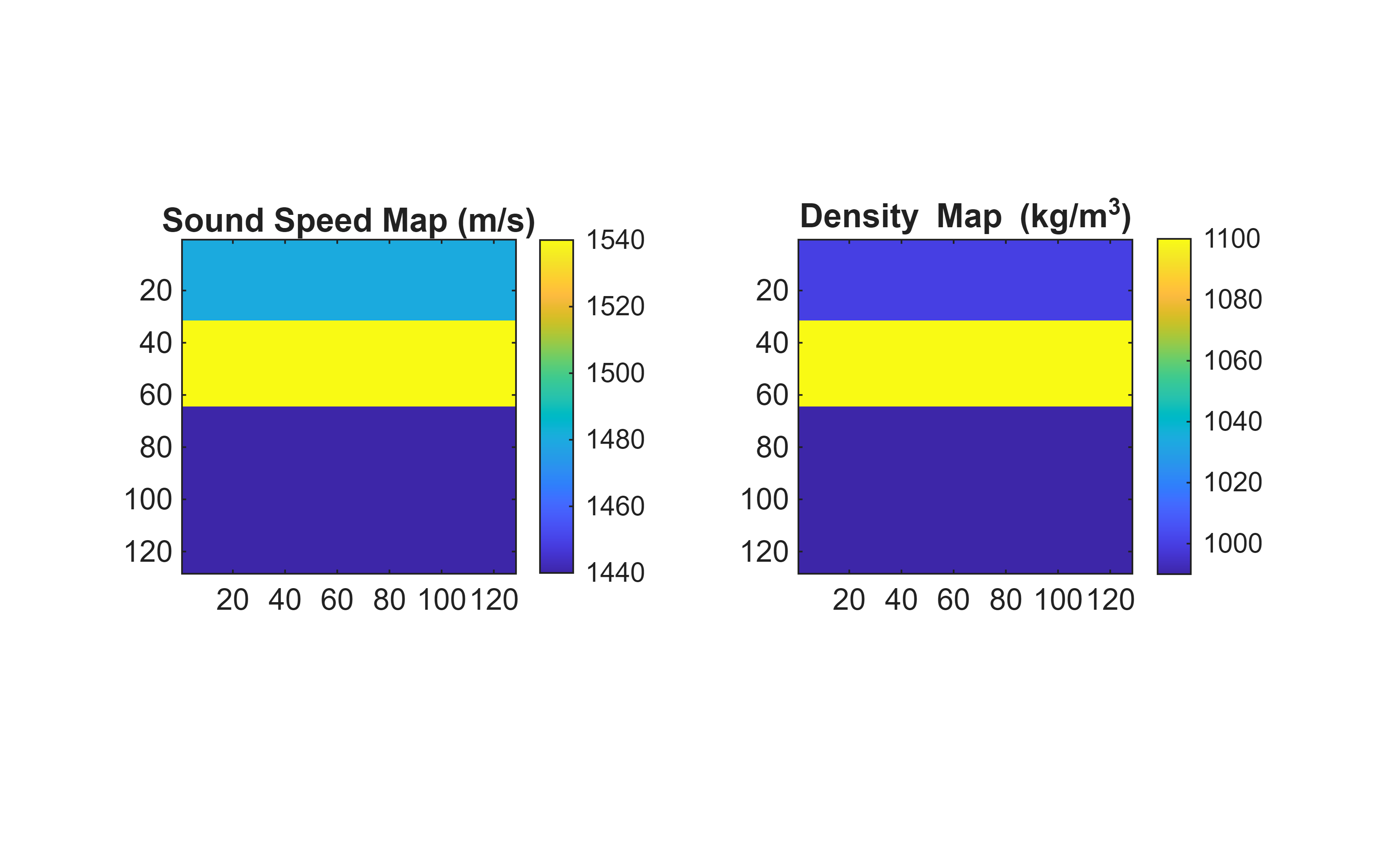
Visualize the sound speed and density maps
Extract the sound speed and density maps
c_map   = medium.soundSpeed;          % [m/s]
rho_map = medium.density;             % [kg/m^3]
Plot the sound speed and density maps
figure;
subplot(1, 2, 1);
imagesc(c_map);
colorbar;
title('Sound Speed Map (m/s)');
axis image;
subplot(1, 2, 2);
imagesc(rho_map);
colorbar;
title('Density Map (kg/m^3)');
axis image;
Define an acoustic source
Create an AcousticSource object
source = AcousticSource(kgrid);
Define an initial acoustic pressure distribution
offset = 0.25*kgrid.dx*Nx;
r = hypot(kgrid.x - offset,kgrid.y);  % radial coordinate
source.initialPressure = exp( -r.^2 / (10*kgrid.dx^2) );
Define an acoustic sensor
Create an AcousticSensor object
sensor = AcousticSensor(kgrid);
Define a binary mask. The solver will return the field variables at the grid locations marked by 1 in the mask, here a line array
sensor.mask = zeros(kgrid.gridSize);
sensor.mask(end - floor(Nx/8),:) = 1;
Run the simulation
Create an AcousticSolver object
solver = AcousticSolver(kgrid,medium,source,sensor);
Define the CFL (Courant-Friedrichs-Lewy) number and endTime allow the timestep to be chosen automatically
cfl = 0.2;
endTime = 0.75 * kgrid.dx*kgrid.Nx / min(medium.soundSpeed(:));
Run the solver
solver.run(CFL=cfl, EndTime=endTime);
Calling kwave.toolbox.AcousticSolver.run...
  Input grid size: 128 by 128 grid points (128 by 128mm)
  Padded grid size: 168 by 168 grid points (168 by 168mm)
  dt: 129.7017ns, end time: 66.6667us, time steps: 514
run completed in 9.7191s
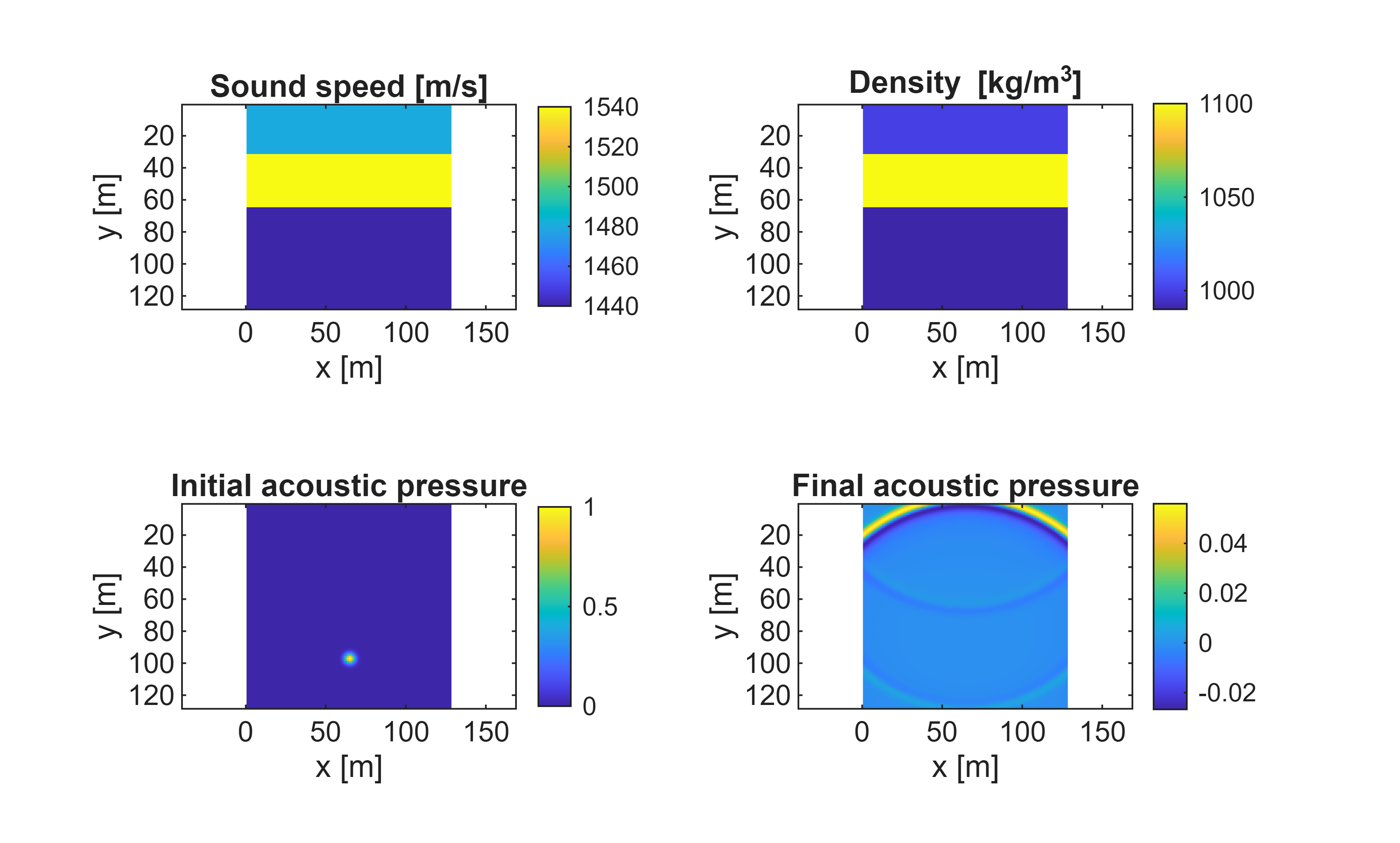
Visualisations
figure
subplot(2,2,1)
imagesc(medium.soundSpeed)
axis equal
colorbar
xlabel('x [m]')
ylabel('y [m]')
title('Sound speed [m/s]')
subplot(2,2,2)
imagesc(medium.density)
axis equal
colorbar
xlabel('x [m]')
ylabel('y [m]')
title('Density [kg/m^3]')
subplot(2,2,3)
imagesc(source.initialPressure)
axis equal
colorbar
xlabel('x [m]')
ylabel('y [m]')
title('Initial acoustic pressure')
subplot(2,2,4)
imagesc(solver.pressure)
axis equal
colorbar
xlabel('x [m]')
ylabel('y [m]')
title('Final acoustic pressure')
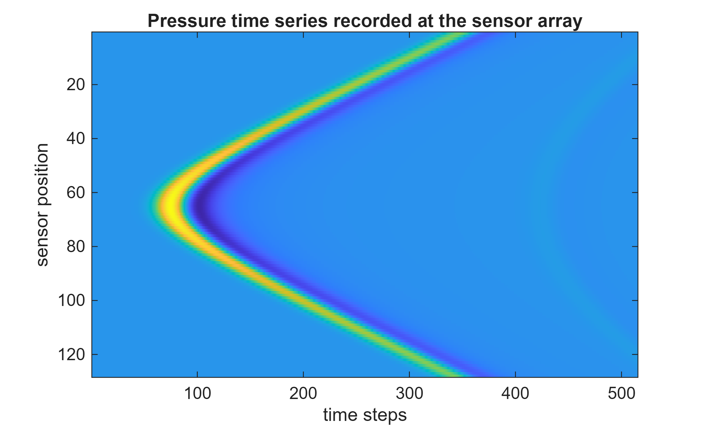
figure
imagesc(sensor.pressure)
xlabel('time steps')
ylabel('sensor position')
title('Pressure time series recorded at the sensor array')