One-Dimensional Acoustic Solver Example
Overview
This simple starter example demonstrates how to construct and run one-dimensional acoustic simulations using AcousticSolver.
- To open the file in the MATLAB Editor:
edit('kwave.tutorials.initialvalueproblems.t01_AcousticSolverExamples1D.m') - To run the file in MATLAB:
run('kwave.tutorials.initialvalueproblems.t01_AcousticSolverExamples1D.m')
See Also:
kwave.tutorials.initialvalueproblems
Preliminaries
This clears the workspace of any old variables
clearvars;
Import the k-Wave-II toolbox
import kwave.toolbox.*
Define a grid
Nx    = 128;          % Number of grid points
dx    = 1e-3;         % Grid spacing [m]
kgrid = Grid(Nx, dx); % Create a Grid object
Define the acoustic properties of the medium
medium = AcousticMedium(kgrid); % Create an AcousticMedium object
medium.soundSpeed = 1500;       % Set a constant sound speed [m/s]
medium.density    = 1000;       % Set a constant density [kg/m^3]
Define an acoustic source
Create an AcousticSource object
source = AcousticSource(kgrid);
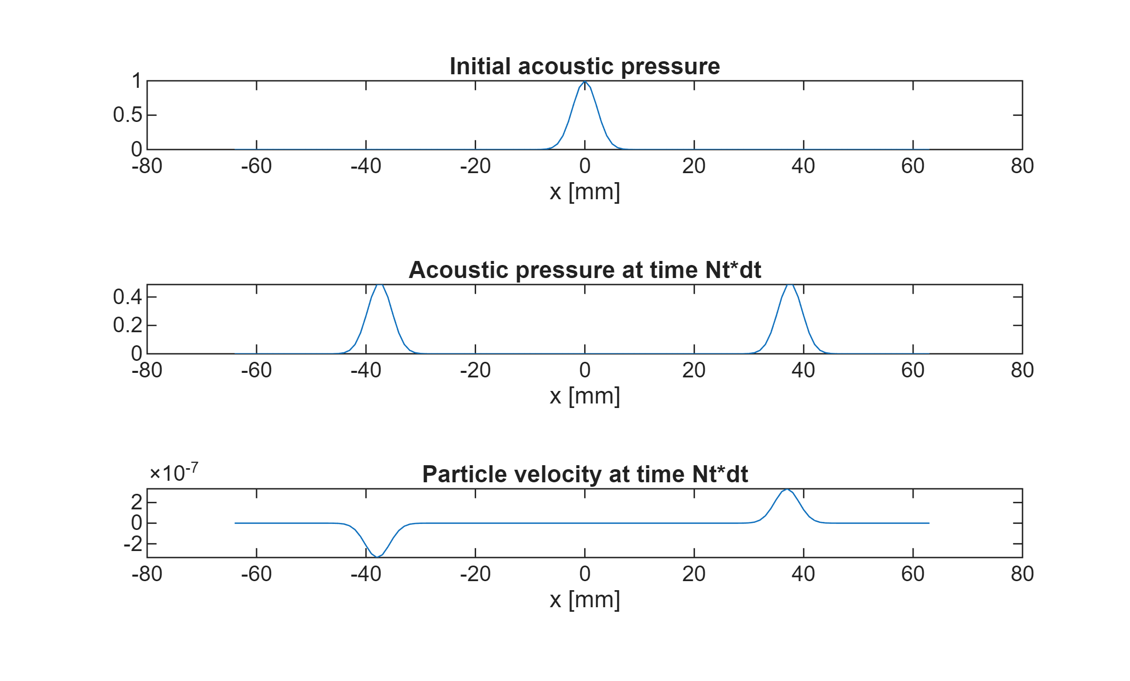
In this example, an initial condition will be used to instigate the acoustic wave. Initial conditions are defined in the AcousticSource class, despite being distinct things mathematically, as they can give rise to an acoustic disturbance. Here the initial acoustic pressure is chosen to be a Gaussian.
source.initialPressure = exp( -kgrid.x.^2 / (10*kgrid.dx^2) );
Run the simulation
To create an AcousticSolver object requires the other objects defined above: kgrid, medium and source. (An AcousticSensor object can be used as the fourth input, but if there are no sensors then it can be omitted, as here.)
solver = AcousticSolver(kgrid,medium,source,[]);
Define the time variables
dt1 = 1e-7; % timestep size [s]
Nt1 = 200;  % Number of timesteps (not including time zero)
Run the solver
solver.run(Nt=Nt1, dt=dt1);
Calling 'run' again will continue the simulation from the end time of the previous run. For example, the following command will take the simulation to timestep 250:
solver.run(Nt=50, dt=dt1);
The same result could have been achieved in one go using:
solver = AcousticSolver(kgrid,medium,source,[]);
solver.run(Nt=250,dt=dt1);
Calling the run function with Nt=0 will not run any additional time steps. If no time steps have been performed, it will just initialise the problem with the initial conditions at time 0:
solver.run(Nt=0, dt=dt1);
Calling kwave.toolbox.AcousticSolver.run...
  Input grid size: 128 grid points (128mm)
  dt: 100ns, end time: 20us, time steps: 200
run completed in 4.1715s
Calling kwave.toolbox.AcousticSolver.run...
  Input grid size: 128 grid points (128mm)
  dt: 100ns, end time: 5us, time steps: 50

run completed in 2.2696s
The simulation output
Following execution of run, the solver object will contain the following output properties:
solver.pressure: A grid-sized arraysolver.densitySplit: A 4D gridfield vectorsolver.velocity: A 4D gridfield vectorsolver.timeArray: A vector of length (Nt+1)
These are, respectively:
- The acoustic pressure field on the grid points at the end time Nt*dt.
- The acoustic density field on the grid points at the final time, split into directional coordinates (for the sake of the PML). The true density field can be found by summing across the 4th dimension.
- The acoustic particle velocity in each of the coordinate directions, evaluated on the staggered grid at time (Nt+0.5)*dt (because of the use of both space and time staggering).
- The time points used in the simulation from time 0 to Nt*dt
Plot the initial and final acoustic pressure fields
figure
subplot(3,1,1)
plot(kgrid.xVec*1e3,source.initialPressure)
xlabel('x [mm]')
title('Initial acoustic pressure')
subplot(3,1,2)
plot(kgrid.xVec*1e3,solver.pressure)
xlabel('x [mm]')
title('Acoustic pressure at time Nt*dt')
subplot(3,1,3)
plot(kgrid.xVec*1e3,solver.velocity)
xlabel('x [mm]')
title('Particle velocity at time Nt*dt')