Two-Dimensional Acoustic Solver examples

Overview

This example demonstrates the AcousticSolver with 2D examples.

To open the file in the MATLAB Editor: edit('kwave.tutorials.initialvalueproblems.t03_AcousticSolverExamples2D.m')
To run the file in MATLAB: run('kwave.tutorials.initialvalueproblems.t03_AcousticSolverExamples2D.m')

Preliminaries

This clears the workspace of any old variables

clearvars;

Import the k-Wave-II toolbox

import kwave.toolbox.*

Define a 2D grid

Nx = 128;      % Number of grid points in x-direction
Ny = 128;      % Number of grid points in y-direction
dx = 1e-3;     % Grid spacing in x-direction [m]
dy = 1e-3;     % Grid spacing in y-direction [m]
pmlSizex = 20; % Thickness of the PML (Perfectly Matched Layer absorbing boundary)
pmlSizey = 20; % Thickness of the PML (Perfectly Matched Layer absorbing boundary)

Create a Grid object

kgrid = Grid([Nx Ny], [dx dy], [pmlSizex pmlSizey]);

Define acoustic properties, and include acoustic absorption

Create an AcousticMedium object

medium = AcousticMedium(kgrid);

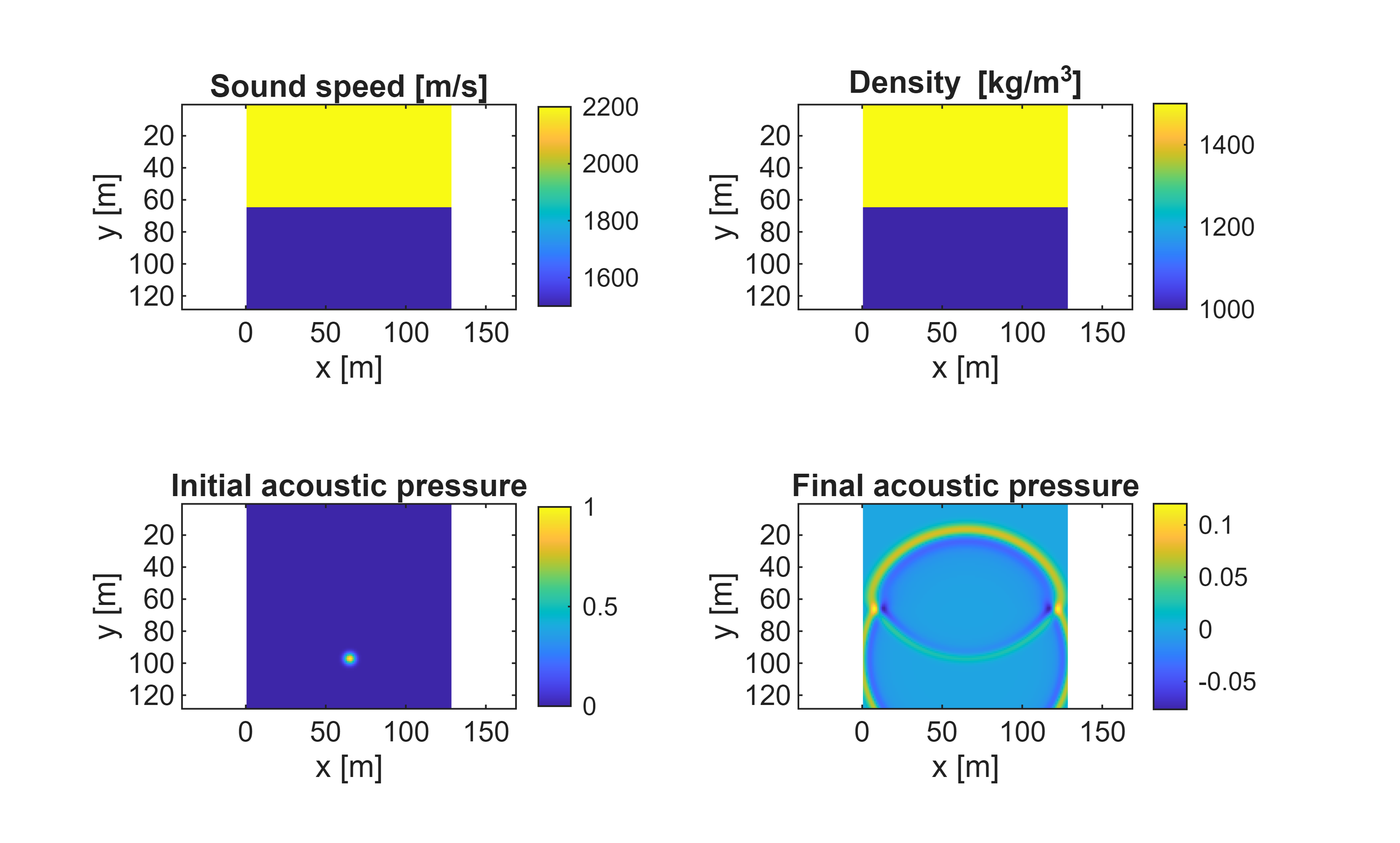
Define a spatially-varying sound speed (here a step change)

c0 = 1500*ones(medium.gridSize);
c0(1:end/2,:) = 2200;
medium.soundSpeed = c0; % [m/s]

Define a spatially-varying ambient density (also a step change)

rho0 = 1000*ones(medium.gridSize);
rho0(1:end/2,:)  = 1500;
medium.density = rho0;  % [kg/m^3]

Define the acoustic absorption coefficient prefactor, the value for alpha0 in the expression for the absorption coefficient: alpha = alpha0 * f^y, where f is the frequency in MHz and y is the power law exponent (absorptionPower, which must be scalar).

medium.absorptionCoeff = 0.5;   % [dB/cm/MHz^y]
medium.absorptionPower = 1.9;

Define an acoustic source

Create an AcousticSource object

source = AcousticSource(kgrid);

Define an initial acoustic pressure distribution

offset = 0.25*kgrid.dx*Nx;
r = hypot(kgrid.x - offset,kgrid.y);  % radial coordinate
source.initialPressure = exp( -r.^2 / (10*kgrid.dx^2) );

Define an acoustic sensor

Create an AcousticSensor object

sensor = AcousticSensor(kgrid);

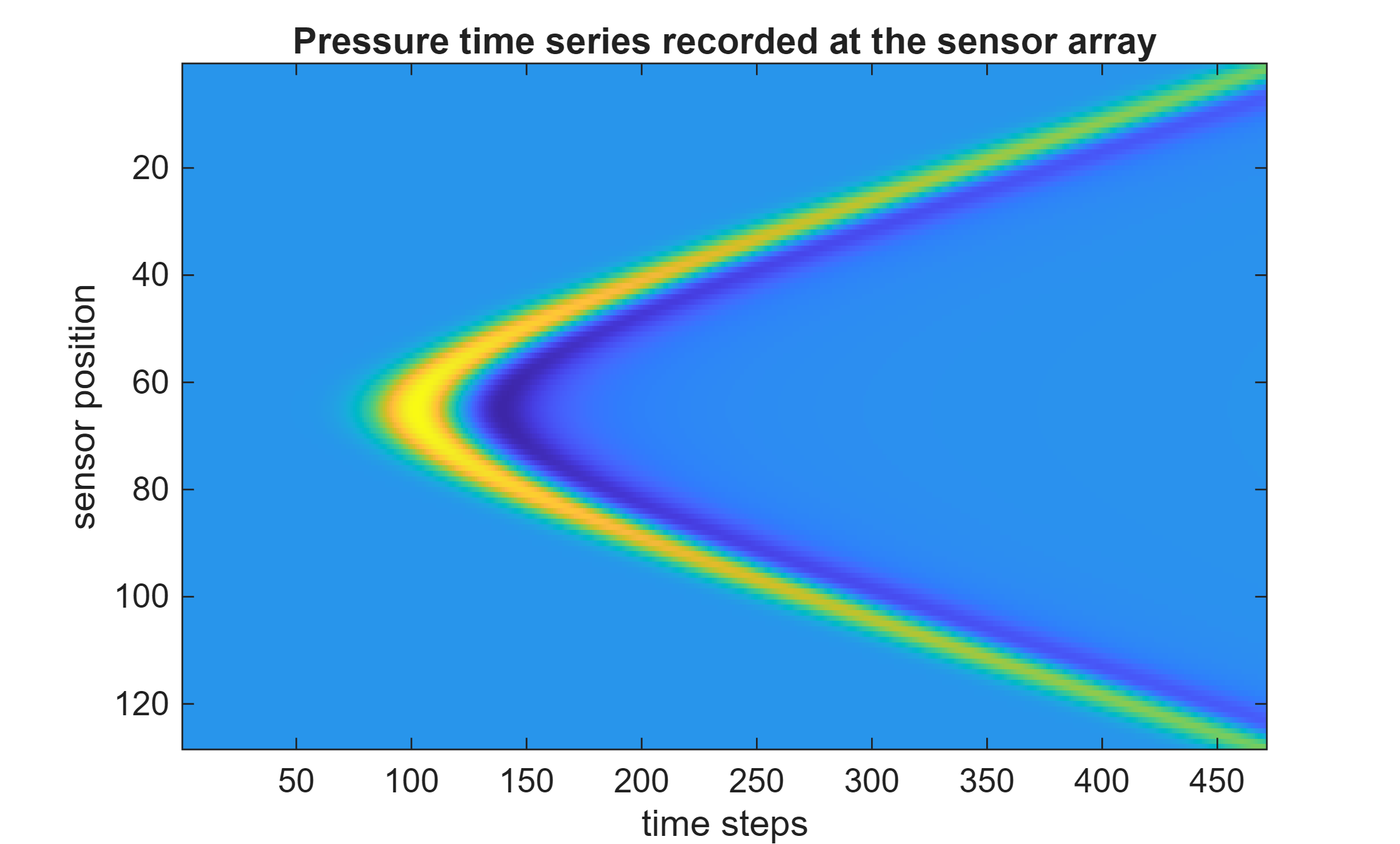
Define a binary mask. The solver will return the field variables at the grid locations marked by 1 in the mask, here a line array

sensor.mask = zeros(kgrid.gridSize);
sensor.mask(end - floor(Nx/8),:) = 1;

Run the simulation

Create an AcousticSolver object

solver = AcousticSolver(kgrid,medium,source,sensor);

Turn on the absorption

solver.absorptionType='on';

Define the CFL (Courant-Friedrichs-Lewy) number and endTime allow the timestep to be chosen automatically

cfl = 0.2;
endTime = 0.5 * kgrid.dx*kgrid.Nx / min(medium.soundSpeed(:));

Run the solver

solver.run(CFL=cfl, EndTime=endTime);

Calling kwave.toolbox.AcousticSolver.run...
  Input grid size: 128 by 128 grid points (128 by 128mm)
  Padded grid size: 168 by 168 grid points (168 by 168mm)
  dt: 90.7801ns, end time: 42.6667us, time steps: 470

  run completed in 13.017s

Visualisations

figure

subplot(2,2,1)
imagesc(medium.soundSpeed)
axis equal
colorbar
xlabel('x [m]')
ylabel('y [m]')
title('Sound speed [m/s]')

subplot(2,2,2)
imagesc(medium.density)
axis equal
colorbar
xlabel('x [m]')
ylabel('y [m]')
title('Density [kg/m^3]')

subplot(2,2,3)
imagesc(source.initialPressure)
axis equal
colorbar
xlabel('x [m]')
ylabel('y [m]')
title('Initial acoustic pressure')

subplot(2,2,4)
imagesc(solver.pressure)
axis equal
colorbar
xlabel('x [m]')
ylabel('y [m]')
title('Final acoustic pressure')

figure

imagesc(sensor.pressure)
xlabel('time steps')
ylabel('sensor position')
title('Pressure time series recorded at the sensor array')